How to create a dynamic drop down list in Excel

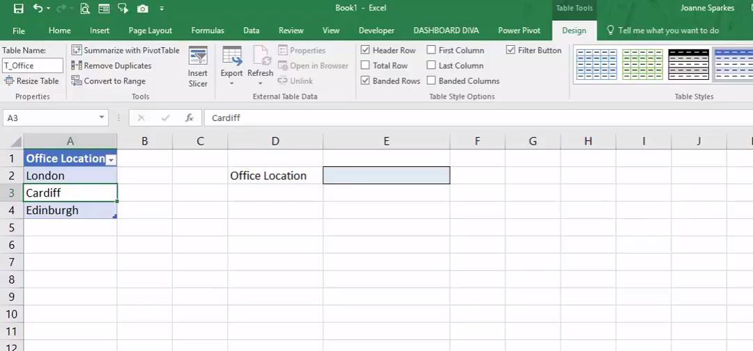
Today I’m going to show you how to create a drop-down list in Excel; and not just any old drop-down list but one where if you change the items in your list, then the drop-down that you’ve created will also change.

You may be familiar with using Data Validation already for creating a dropdown list. If not, then to create a dropdown click in a cell where you want to have a list appear, choose the Data tab and then Data Validation. Click List and then create a source for your list.

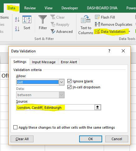
You might type the items in, so e.g. type London, Cardiff, Edinburgh and click OK,

When you choose the cell containing the list you will see the items appear.

Using this method, then if you wanted to add some more items, you’d have to go back into Data Validation and recreate the list all over again. If you wanted to reorder them, you’d have to do the same. You could create a named range in your worksheet, or select a range of cells, but then that range stays the same size and isn’t easy to alter.

What I’m going to show you how to do is make it so that this is a little bit more flexible.

First we’re going to do is change this list into a table. To do that you can either highlight the list, go to Insert and Table, or the way I like to do it is just to press Ctrl T on your keyboard, which is the shortcut, and it will ask where your data is.

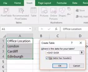
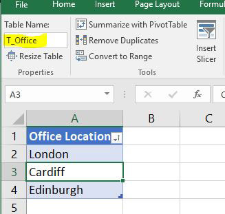
My table has got a header in it, Office Location, so I’m going to tick “My table has headers” box and click OK. You’ll see that you now have a little list that’s been highlighted in the default colours in your Excel and it’s now a table. If I click inside it, you’ll see the design options for our table come up. I’m going to give it a name that I can remember, so I’m going to call it T_Office, and press return. Now, we’ll always be able to find it.

If you start to write a formula using a table column, you’ll see something quite special about them.

If, for example, I try to create a formula by typing = then clicking and dragging down from cell A2 to A4, then instead of the range details appearing in the formula bar you’ll see that the name of the table, T_Office, followed by the column that you’re looking at.

=T_Office[Office Location]

I’m going to use these words in another formula, so go to the formula bar, highlight then phrase and copy using Ctrl C.

Go to the Formula tab and click on Name Manager. Click Add to enter a new name.

We’ll call it R_Office this time. Where it says Refers To, the formula we’re going to use is:

=INDIRECT(“T_Office[Office Location]”)

Click Close.

Now, back to our Data Validation. Click back where we want our drop-down box to appear, click on Data, then Data Validation, and now where it says List, change the source to

=R_Office

and click OK

Now, we’ll see that we’ve got London, Cardiff, Edinburgh in the list and it’s picking up the whole column of the table to use as the dropdown.

What is quite special about this now is if I were to add another office to the list, let’s say I’ve opened another one in Birmingham, I’d type it right under the last name that appears. You’ll see that the table automatically expands to include the new office.

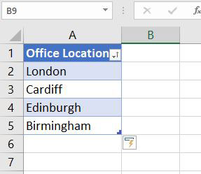
You don’t have to have the table of dropdown items and the cell with the dropdown on the same sheet. You could put your lookups on a totally different worksheet if you wish,

Wherever it is, you’ll find that as you update your items in the table then your dropdown will automatically update with all the latest information.

We could also sort our office list. Click anywhere on the table column, and on the data tab, click sort A to Z.

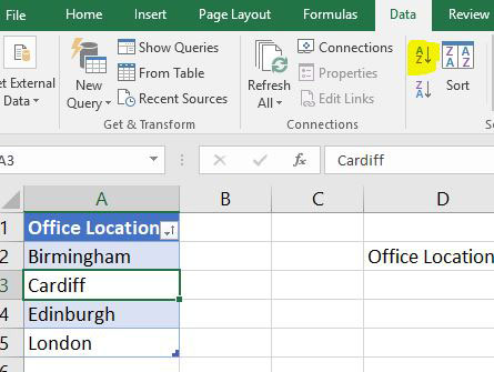
That list is now ordered alphabetically, and what we should find when we click in our Office Location drop-down is that this is also sorted alphabetically.

So, whatever you do now to this table will be reflected in your drop-down.

and that’s it.